on
Economic Forces
This week, we looked at using various economic variables as predictors for election outcomes. In this blog, I aim to predict Republican seat share and incumbent party vote share using variables such as GDP growth percentage, CPI percent change, disposable income percent change, and the national unemployment rate.
So far, we have touched on a few different forces that affect the way in which people vote – aside from simply party affiliation. Last week, we learned about end heuristics, or how voters tend to focus on the period of time right before an election rather than an incumbent’s entire time in office. If the candidate ends their term strong, that is what people are likely to remember. I have brought that idea into this week’s analysis of economic forces – choosing to focus on Quarter 7, or July through August in an election year.
According to Lewis-Beck and Stegmaier (2000), voters tend to weigh economic issues more heavily than other issues, and they “hold the government responsible for economic performance”. While the government can only do so much to mitigate the economy’s natural cycles, people still hold those in office responsible for it all. It should also be noted that Republicans give more weight to economic issues than Democratic voters. The economic variables that I will consider in this analysis are GDP growth percentage, percent change in disposable income, percent change in Consumer Price Index (CPI), and the national unemployment rate.
In order to make predictions, I have created four different linear regression models that build off of one another in the variables used to predict the incumbent party’s vote share percent. The first starts off with only GDP growth percent as an independent variable, and we find this is not a good model for prediction. As shown in the regression table under “Model 1”, the coefficient on GDP growth is insignificant and the model has an R-squared value of 0.00, telling us that 0% of the variation in incumbent party vote share can be explained by GDP growth percent in this model. This model does not fit the data well at all.
We expand on this model by then adding an independent variable for the percent change in disposable income (Model 2), and then, in a different model, another independent variable for the unemployment rate (Model 3). In both of these models, all the independent variables’ coefficients remain insignificant, although we do see a slight rise in the R-squared value. In Model 2, the R-square value is 0.02, and in Model 3 it is 0.04. While this shows a slight increase from Model 1, these numbers are still indicative of a model that does not fit the data well at all.
In the final model, I added an independent variable for the percent change in CPI. Here (Model 4), this CPI variable is significant at the 5% level. For every 1% change in CPI, the incumbent party vote share percent increases by 1.55 on average. In a healthy economy, some inflation is expected, so this increase in CPI leading to an increase in the incumbent’s vote share percent could indicate that people see rising prices as a positive thing. This model also has an R-squared value of 0.23, showing that it is a much better fit for the data than the previous three models. I coded the CPI percent change variable by changing the monthly CPI statistic into a quarterly average, and then created the CPI change variable by lagging the CPI from the previous quarter and converting it into a percent change with respect to that quarter’s CPI. I believed this would give an accurate representation of inflation in the economy, and is more understandable than the CPI index number that shows the price of a specific basket of goods.
While the relationship between CPI percent change and vote share is positive in this model shows, current events could change this relationship, or at least create an inflation threshold where it goes from being seen as a good thing to a bad thing. Our inflation levels are so high right now that the CPI index is likely negatively correlated with how the incumbent party will do in the upcoming election.
Looking at the variable on GDP growth percentage, it is counterintuitive for the coefficient to be negative. One would think that when GDP is increasing – a sign that the economy is doing well – the incumbent would do better in the election. This variable is very low in magnitude, however, so should not affect the predictions much. This strange outcome could be the result of multicollinearity, which I will touch on later in this post.
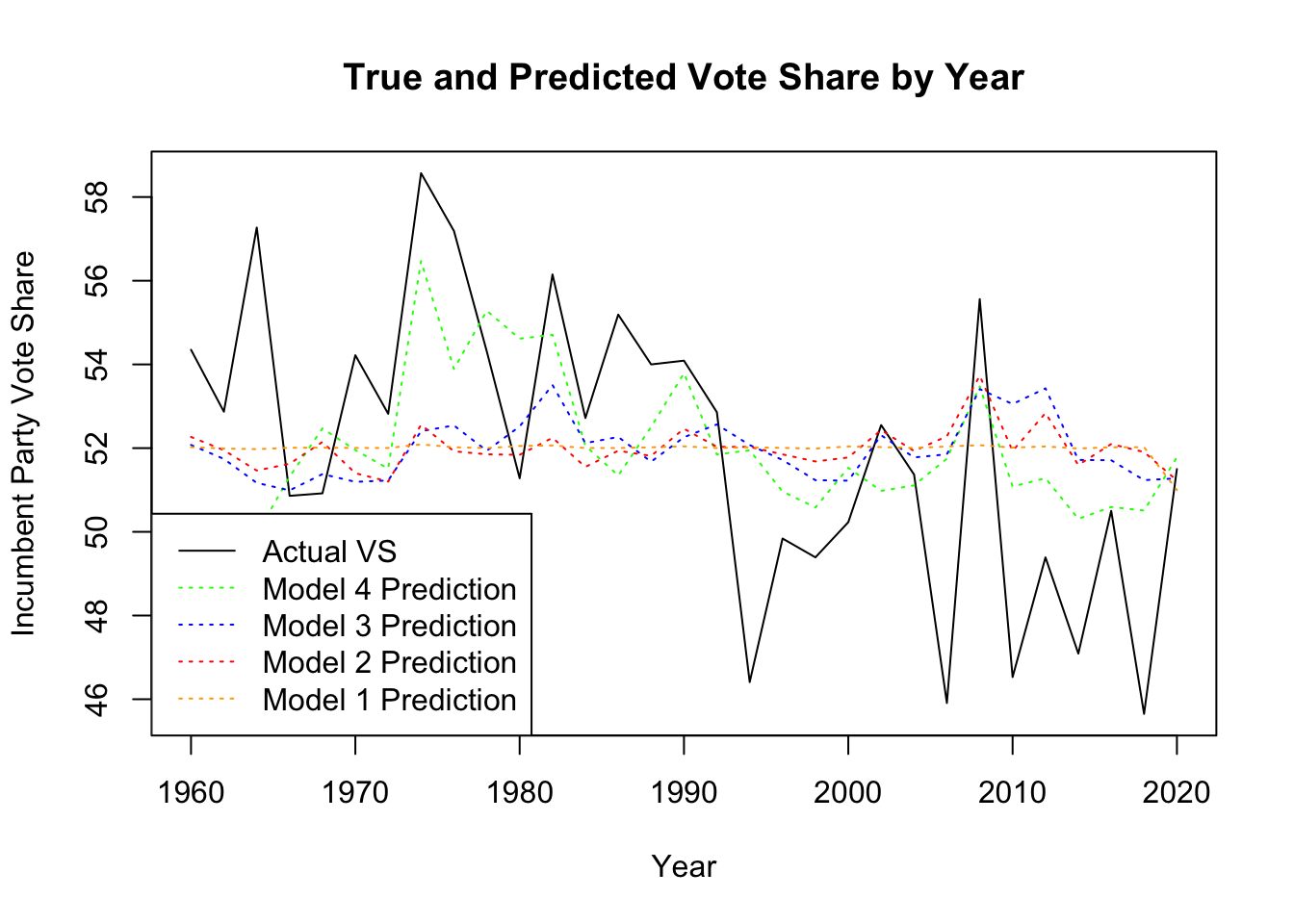
To look at how these models fit over time, I created a graph that shows each model’s predictions alongside the actual values of incumbent party vote share. Each model is a colored, dotted line, while the actual values are represented by the black, solid line. As we can see, all of the colored lines do not have as much variation as the true values line; they are all much flatter. Only the green line representing Model 4 comes close to following the patterns of the actual vote share values, but even it cannot recreate the variation we see over time. This model that used CPI did a decent job of predicting between 1970 and 2000. After 2000, however, it did not hit the lows that we saw with the actual values. Until the 1990s, incumbent vote share typically sat above 52%. After this period and into the 2000s, however, the incumbent was not as successful, often falling into the mid 40-percents. It is during this time period that the residuals appear to grow.
| Dependent variable: | ||||
| H_incumbent_party_majorvote_pct | ||||
| (1) | (2) | (3) | (4) | |
| GDP Growth Percentage | -0.045 | -0.163 | -0.196 | -0.080 |
| (0.157) | (0.229) | (0.235) | (0.219) | |
| Disposable Income Percent Change | -0.565 | -0.452 | -0.008 | |
| (0.794) | (0.814) | (0.764) | ||
| Unemployment Rate | 0.323 | 0.200 | ||
| (0.419) | (0.386) | |||
| CPI Percent Change | 2.392** | |||
| (0.950) | ||||
| Constant | 52.046*** | 52.455*** | 50.480*** | 48.563*** |
| (0.660) | (0.880) | (2.706) | (2.587) | |
| Observations | 31 | 31 | 31 | 31 |
| R2 | 0.003 | 0.021 | 0.042 | 0.230 |
| Adjusted R2 | -0.031 | -0.049 | -0.065 | 0.111 |
| Residual Std. Error | 3.494 (df = 29) | 3.524 (df = 28) | 3.550 (df = 27) | 3.243 (df = 26) |
| F Statistic | 0.084 (df = 1; 29) | 0.295 (df = 2; 28) | 0.393 (df = 3; 27) | 1.939 (df = 4; 26) |
| Note: | p<0.1; p<0.05; p<0.01 | |||
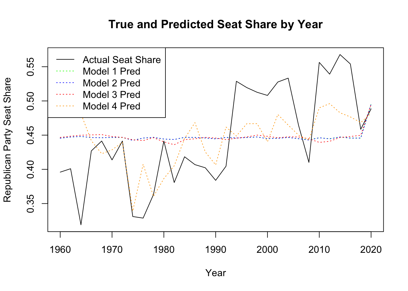
I repeated this modelling process and prediction but instead using Republican seat share percentage as the dependent variable. The first three models that do not use CPI percent change again came up poorly fitting models for the data, with no significant independent variables. Only once percent change of CPI is added does the model have a relevant r-squared value of 0.30, and the CPI dependent variable is significant at the 1% level. These models demonstrate the same effects for incumbent vote share as for Republican seat share.
Once again, I created a plot of the predictions versus the true values over time. Interestingly, we see the same pattern of the CPI model fairly accurately fitting the actual values until the 1990s, after which they diverge and the residuals grow. The other three models appear as flat lines in this graph, similar to the plot above.
| Dependent variable: | ||||
| RepSeatShare | ||||
| (1) | (2) | (3) | (4) | |
| GDP Growth Percentage | 0.002 | 0.002 | 0.002 | -0.001 |
| (0.003) | (0.005) | (0.005) | (0.004) | |
| Disposable Income Percent Change | 0.0002 | -0.001 | -0.012 | |
| (0.017) | (0.017) | (0.015) | ||
| Unemployment Rate | -0.002 | 0.001 | ||
| (0.009) | (0.008) | |||
| CPI Percent Change | -0.061*** | |||
| (0.019) | ||||
| Constant | 0.445*** | 0.444*** | 0.456*** | 0.505*** |
| (0.014) | (0.018) | (0.057) | (0.052) | |
| Observations | 31 | 31 | 31 | 31 |
| R2 | 0.016 | 0.016 | 0.017 | 0.299 |
| Adjusted R2 | -0.018 | -0.055 | -0.092 | 0.191 |
| Residual Std. Error | 0.073 (df = 29) | 0.074 (df = 28) | 0.075 (df = 27) | 0.065 (df = 26) |
| F Statistic | 0.458 (df = 1; 29) | 0.221 (df = 2; 28) | 0.158 (df = 3; 27) | 2.773** (df = 4; 26) |
| Note: | p<0.1; p<0.05; p<0.01 | |||
One issue to note when analyzing the effects of different economic forces jointly on a dependent variable is multicollinearity. This is a problem that occurs when multiple independent variables are correlated with one another and negatively impacts the reliability of the inferences we can draw from these models. To assess if multicollinearity exists between any of the independent variables, I have created a correlation matrix below.
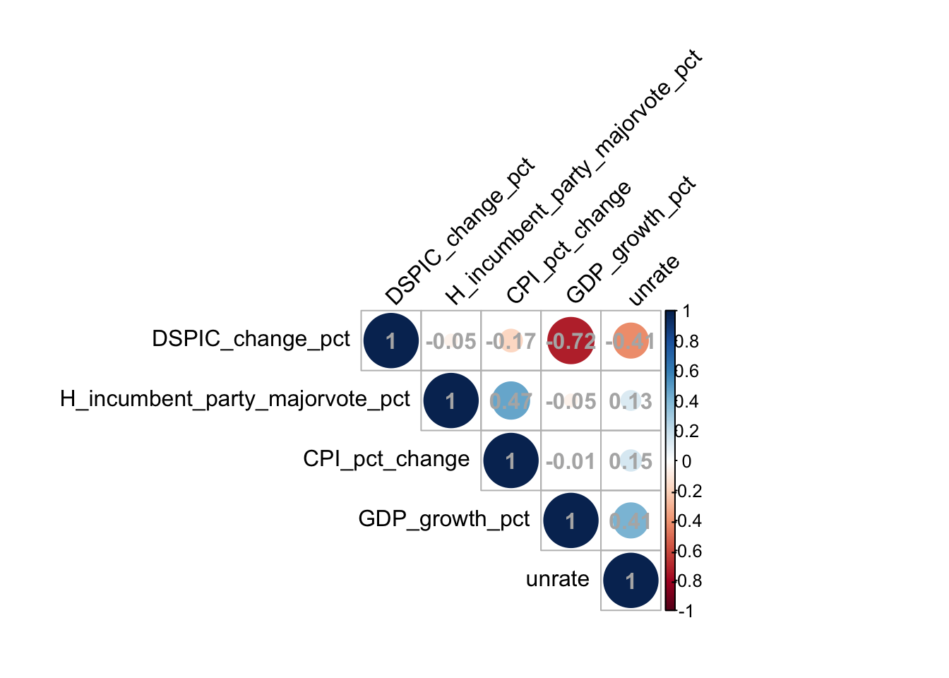
We can see that GDP growth percentage is highly negatively correlated with the percent change in disposable income, with a correlation of -0.72. There is also a moderately strong correlation between the unemployment rate and the percent change of disposable income. Both of these correlations may impact the validity of our models and hurt any insights we draw from this analysis.
Finally, below is my prediction of vote share for the incumbent party in the house using 2022 Q6 data. While the model I fit used Q7 data, we are currently in the middle of Q7, so this information was not readily available. There will naturally be some limitations with this prediction due to this simple fact. Additionally, since the model relies so heavily on CPI percent change, the prediction is likely an overestimate of the incumbent vote share. I believe the relationship between CPI percent change and incumbent vote share is likely not linear, and with the levels of inflation that we have seen over the past year, this variable brought the prediction way up when it likely should have brought it down a little bit.
##       fit      lwr      upr
## 1 55.2138 44.76077 65.66684