on
Shocks
This blog is part of a series related to Gov 1347: Election Analytics, a course at Harvard University taught by Professor Ryan D. Enos.
This week we learned about how the things we cannot predict happening can end up affecting election outcomes. Shocks capture everything from natural disasters and Supreme Court decisions to e-mail scandals and sports outcomes. While no one expects these events to happen, voters sometimes blame candidate losses on these shocks. We will look to explore the true effect of these political shocks, or lack thereof, on elections.
During an election year, there are always unexpected stories to come out about candidates, business cycle swings, or other shocks that can influence voters at the polls. Incumbents can pay the price when things in the world are going wrong, like sports teams losing or rainy weather, regardless of whether or not they have anything to do with it. For example, Achen and Bartels concluded that shark attacks in New Jersey reduced Woodrow Wilson’s vote share by ten percentage points. While Fowler and Hall contest this finding, the impact of shocks on politics is a continuing debate.
The effects of these shocks on candidate support may bear more meaning during a national election, but they may also affect sentiments toward each party in terms of a generic ballot. We know from previous analyses that the generic ballot is a decent predictor for House elections, so exploring how shocks influence house elections with the thought of possibly accounting for them in our predictive models is a reasonable inquiry.
There have been several shocks so far in 2022, some very political, such as the Dobbs Supreme Court decision on abortion, historic levels of inflation, a student-loan forgiveness plan introduction, and more. In class we saw how the Dobbs decision was covered in the news and how it affected party sentiments, with Republican support declining and Democratic support increasing in the aftermath. In an extension on this, I want to see how the economic shocks we experienced in the US this past summer influenced party support. On July 13th, the Bureau of Labor Statistics reported inflation data from June, recording a consumer price index (CPI) of 9.1% from the year prior - a figure that hadn’t been seen since 1981. With a Democratic president in office, some people placed the blame of this increased cost of living on President Biden and his party.
By scraping the New York Times articles, we can see below the number of articles that used the word “inflation”, with the vertical line marking the day that the BLS reported the inflation statistic to the public.
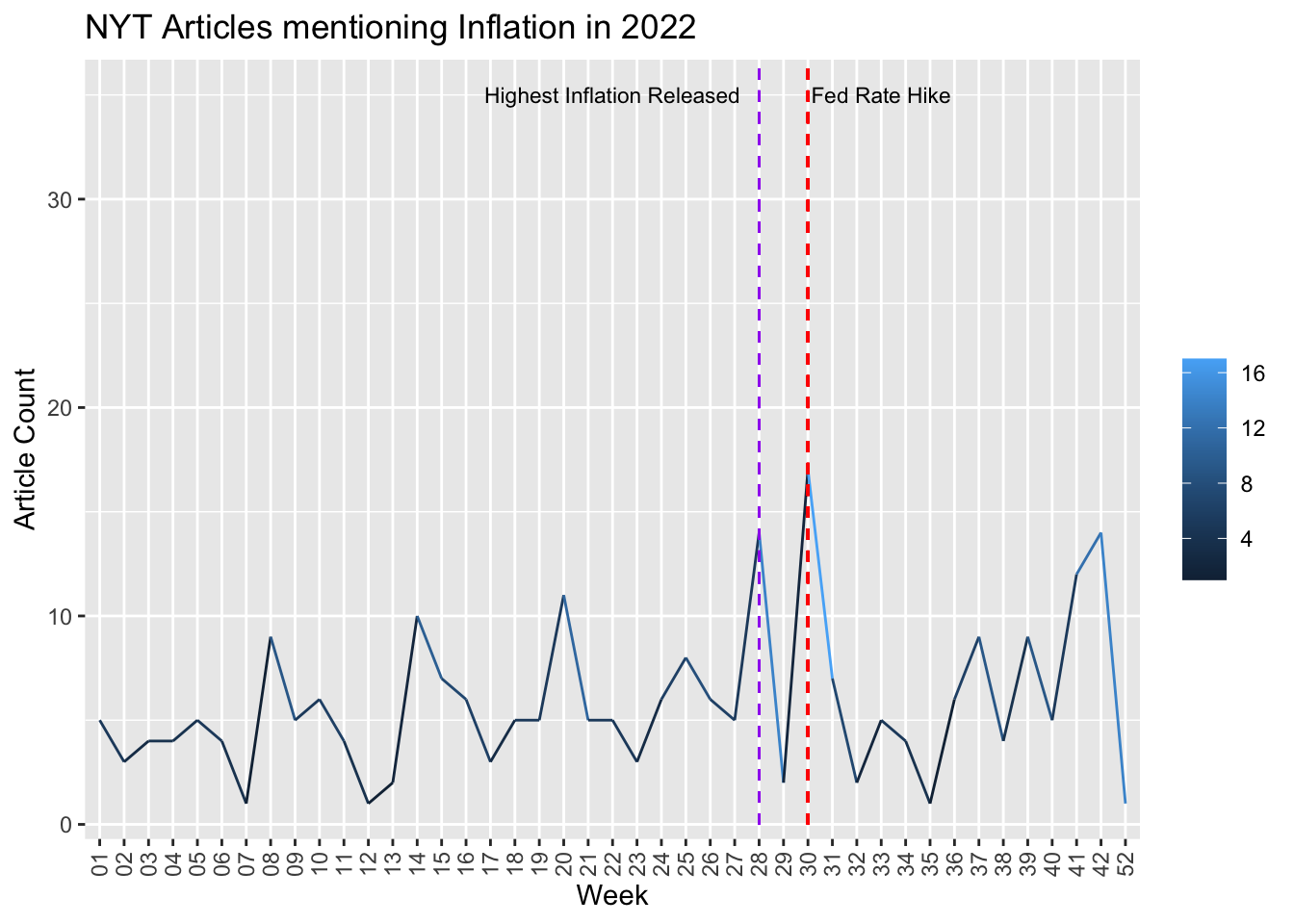
We can see a spike in the number of articles on that day, but we also see other spikes falling at regular intervals earlier in the year as well - weeks 8, 14, and 20. After some further investigation, it seems that these were also around the times when the BLS released the prior month’s CPI. The spike of articles during the week of July 13th, when the high inflation was first reported, is not that much higher than in the year’s prior spikes, we see another spike almost immediately following, in week 30, or July 24th-30th. This was the week when the Fed announced their interest rate hike that was to curb inflation. In analyzing the frequency of the word “inflation” in articles, we not only capture the shock of the summer’s high CPI, but also the shock of the Fed’s decision.
Now in looking at how both of these impacted party sentiments: below we mark these dates on a graph of the generic ballot over time.
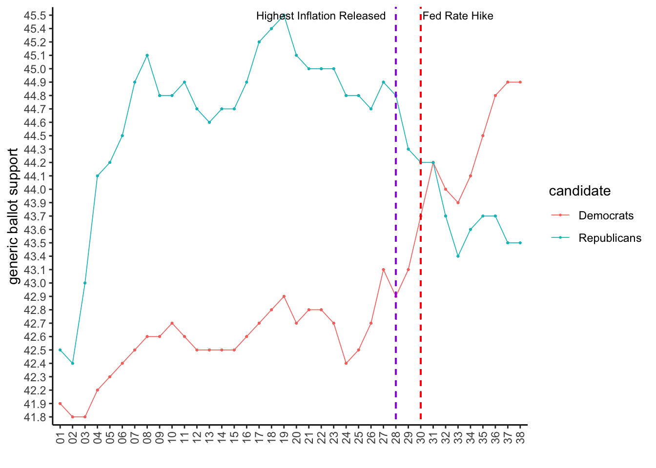
We can see that when the report of inflation reaching 9.1% in June was released, The Republican party support was already on a decline and continued to decline further. We also see the exact opposite with the Democratic party, where support was already on the rise and it continued to rise. This is slightly counter-intuitive to the effect we would have expected to see with a shock of this nature. Given that the government at the time of this inflationary period is controlled by Democrats, we would have expected to see support for Democrats to decrease after this news, but we see the exact opposite. When the Federal Reserve hiked the interest rates in late July, we see the same trend of decreasing Republican support - but with a short plateau period immediately following this news break. However, we also see Democratic support fall a week after this too. While this graph can be picked apart and inferences can be made about how these shocks impacted party support, it seems that these trends are the result of larger forces. There are many shocks that took place over the course of this year that may have impacted the generic ballot, or there may just be generally changing sentiments about the parties throughout the country that have no rhyme or reason and lead to these fluctuations. It is also worth noting that the y-axis range is around 4 percentage points, meaning these fluctuations are not nearly as large as the graph may make them appear.
From this analysis in addition to class to class discussion, it does not seem like we can accurately measure the effect of a single shock on party sentiments or election predictions. There will always be shocks and they occur frequently, but their effect is temporary. News outlets may place blame on a shock for the outcome of an election to stir up a story, but it is impossible to determine whether or not a shock cost a candidate an election.
Model
Over the past few weeks, we have tested out adding different pieces of election data to our models to see if they will yield more significant results and improve our predictions for this year’s election. Some of these attempts showed real predictive power, like the generic ballot and real disposable income changes, while some of the data fell short of what we had hoped, such as that on advertising. In adjusting my model this week, I will stick to the fundamentals of incumbency, economic variables, and turnout to see if my model has improved. I will try new combinations of variables, weights, and methods to hopefully improve upon this model.
Throughout my models in previous weeks, I have found a few variables to be consistently significant and therefore will keep them in my model. Similar to in previous weeks, Democratic vote share will be the dependent variable of the model. We will also use democratic vote share from the previous election as an independent variable, along with unemployment rate in Quarter 7, the President’s party, the House’s majority party, the generic ballot, and voter turnout.
| Dependent variable: | ||||||
| DemVotesMajorPercent | ||||||
| (1) | (2) | (3) | (4) | (5) | (6) | |
| gen_avg_dem | 0.636*** | 0.445*** | 0.587*** | 0.232*** | 0.182*** | 0.425*** |
| (0.015) | (0.010) | (0.049) | (0.038) | (0.039) | (0.040) | |
| inc_partyR | -36.312*** | -33.163*** | -15.649*** | -15.613*** | -15.447*** | |
| (0.074) | (0.177) | (0.181) | (0.180) | (0.179) | ||
| president_partyR | 3.205*** | 2.263*** | 3.714*** | 4.916*** | 0.652** | |
| (0.076) | (0.185) | (0.145) | (0.227) | (0.295) | ||
| dist_turnout | -9.802*** | -4.566*** | -5.400*** | -7.518*** | ||
| (0.736) | (0.578) | (0.590) | (0.593) | |||
| lag_DemVS | 0.567*** | 0.565*** | 0.572*** | |||
| (0.004) | (0.004) | (0.004) | ||||
| Q3_unemployed | 0.348*** | 0.150*** | ||||
| (0.051) | (0.051) | |||||
| H_incumbent_partyR | 5.114*** | |||||
| (0.228) | ||||||
| Constant | 22.907*** | 44.884*** | 42.274*** | 19.509*** | 19.656*** | 8.795*** |
| (0.701) | (0.485) | (2.125) | (1.669) | (1.668) | (1.725) | |
| Observations | 206,336 | 206,336 | 36,212 | 35,887 | 35,887 | 35,887 |
| R2 | 0.009 | 0.543 | 0.503 | 0.699 | 0.699 | 0.703 |
| Adjusted R2 | 0.009 | 0.543 | 0.503 | 0.699 | 0.699 | 0.703 |
| Residual Std. Error | 24.327 (df = 206334) | 16.510 (df = 206332) | 16.585 (df = 36207) | 12.948 (df = 35881) | 12.940 (df = 35880) | 12.850 (df = 35879) |
| F Statistic | 1,816.863*** (df = 1; 206334) | 81,861.170*** (df = 3; 206332) | 9,168.786*** (df = 4; 36207) | 16,634.830*** (df = 5; 35881) | 13,888.080*** (df = 6; 35880) | 12,142.990*** (df = 7; 35879) |
| Note: | p<0.1; p<0.05; p<0.01 | |||||
Looking at the R-squared and adjusted R-squared values of each of these models, we see that they increases when we add the lag of Democratic vote share in Model 4, however in Models 5 and 6 that follow both add variables that barely have any affect on the R-squared, raising it only by 0.001. These variables are unemployment in Q3 before an election, and whether the house was controlled by a democrat or a republican majority. While these two variables do not have much impact on the R-squares, they are shown in the model as being statistically significant at the highest level.
To test for multicollinearity between these independent variables, I have created the correlation plot below.
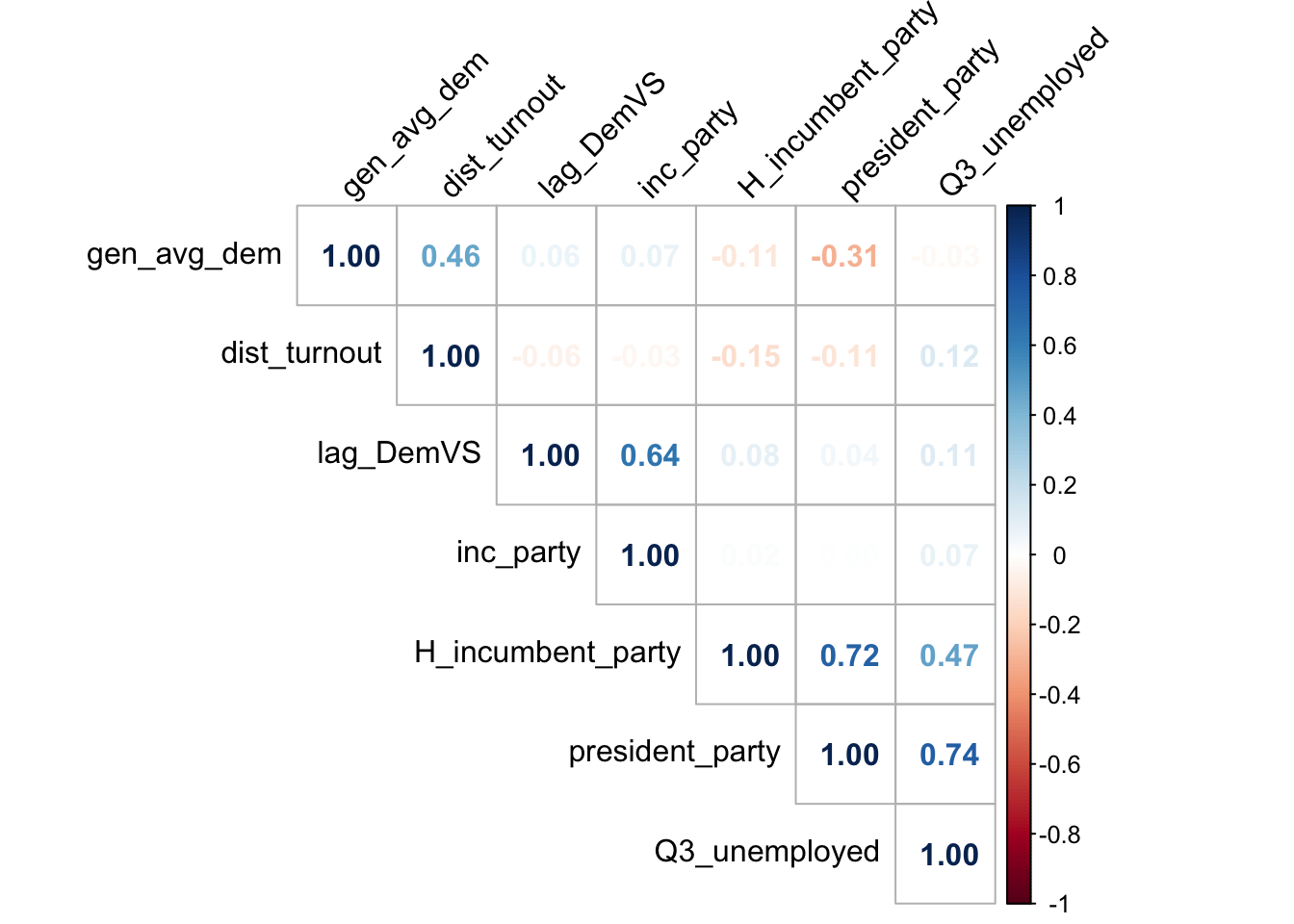
We can see that, for the most part, the variables have very low correlation with one another. We do see a high correlation of 0.74 between the President’s party and the Q3 unemployment rate, and a correlation of 0.72 between the president’s party and the house incumbent party. In both of these highly correlated relationships, it is hard to believe that there are unaccounted for variables that explain this phenomenon. For example, while presidents can have some impact on the economic climate, their party is wholly uncorrelated with the business cycle swings that are a strong determinant of unemployment rates. Looking at the second relationship, we learned in class that there exists a phenomenon where the house majority party will switch at the midterm after the president party switches, therefore they may exist a linear relationship between these two variables. As I discussed earlier, the variables of the House’s incumbent party and the Q3 unemployment do not improve the predictive power of the model, so to eliminate this multicollinearity, we can shift to only looking at Model 4.
We also see a somewhat high correlation between the lag of democratic vote share in the district and the seat’s incumbent party. It makes sense that a relationship exists between these two because they are both looking at the outcome of the previous election cycle. If the district’s incumbent was a democrat, we can expect that the district would also have a higher democratic vote share. Adding the lag democratic vote share variable did increase the R-squared value by a decent amount, as did the seat’s incumbent party. In future weeks I will look into this relationship further to determine if one of these variables should be eliminated from the model.