on
Final Prediction
This blog is part of a series related to Gov 1347: Election Analytics, a course at Harvard University taught by Professor Ryan D. Enos.
Over the past nine weeks, we have explored a multitude of variables that may impact election outcomes in an attempt to forecast the 2022 midterm election. We have learned about economic forces, polling, expert predictions, incumbency, advertising, campaigning, and more to find if they hold any predictive power, and how together in a model they may foreshadow what is to come in the results next week. In this blog, I will create a final prediction model for the House of Representatives and share its results, with the intention of reflecting on it after the election.
Background
Since this class first convened in the beginning of September, we have time and time again been reminded of the shortcomings of election forecasting. Elections are fickle and there is no way to know for certain how voters will vote on election day. The experts oftentimes cannot predict what will happen, if an election will be toss-up or a landslide. There are shocks that no one sees coming, costs of voting that may be unanticipated, various biases with polling, and ever-changing political opinions that result from all sorts of issues and news. While these unknowns make forecasting very difficult, we have gained the tools over the last nine weeks that give us a good foundation to create predictions of our own for the House of Representatives midterm election.
My Model Choices
In building my model, the first choice I had was what to use as my dependent variable and the level on which to predict on. For my dependent variable, I decided to run models for both Democratic seat share and Democratic vote share to see the results of both and how they may unveil different stories about the election. I also created variables putting the vote share and seat share in terms of the incumbent party to see how incumbents perform without paying specific attention to their party affiliation, but I decided that this approach would complicate interpreting results. While we spent multiple weeks working with district-level data and forecasting each of the 435 districts, in the end I have decided to predict vote share and seat share on the national level. We have more data for these variables and do not have to rely upon things like pooling, that may produce greater margins for error. Given the insufficient district-level data, a pooled model would have allowed us to take data from neighboring, similar districts and count it as its own. However, my national model was heading in the right direction in terms of improving predictability, and the lack of district data led me to decide on a national-level final model.
In the first week of class, we looked at the fundamentals of election forecasting models, with predictors like the president’s party. We learned about the phenomenon that takes place in most midterms where the president’s party tends to lose seats (Campbell 2018). Following these basics, in week two we looked at how Real Disposable Income (RDI) on its own does a decent job of predicting elections. We also took a look at a slew of other economic variables, such as the Consumer Price Index (CPI), GDP growth rate, unemployment, and more. Despite the overlap between the government and the economy, most of these variables proved to be insignificant and poor predictors for the House elections. The one economic variable I will be using in my final model the unemployment rate, as it is typically a decent indicator of the health of the economy. In addition to using it on its own, I have also decided to interact it with the president’s party. The most important topics to voters vary based on their political party affiliation, and Republicans are known to weigh economic factors more heavily. Therefore, an interaction term between party and unemployment rate can provide us with more significant results than the two can separately on their own.
We continued on from the fundamentals and economic variables onto polling, looking at the generic ballot as well as district-level polls. When adding these polls to my model, I had limited the data to 1990 and later, justifying this with the fact that polling methods have greatly changed since 1945 when the data was first captured. It was my hope that in reducing the sample, the model would better predict recent elections. While I think this justification still makes sense, especially for district-level polling where there does not exist much data even today, I will not be limiting the data by year as severely. In my final model, the only polling data I will be using is the generic ballot, measuring which party people support without regard for specific candidates. The data I will be using goes back to 1960, which is when all the variables of my interest have data for. It would still make sense to limit the data to more recent years for the same polling reasons, but since I am only dealing with the generic ballot, I believe the changing polling methods will not hinder the predictability of the model and it will be more useful to have the longer data.
While we did not dedicate much time in class to discussing presidential approval ratings and their impact on elections, some classmates and I spoke about incorporating it as another form of polling that has easily accessible historical data. I gathered data on presidential approval from Gallup Analytics that date back to 1960. Polling dates varied year to year, so I decided pulled the president’s approval rating from whichever the last poll right before the election was. A few years in the 1960s and 1970s, this ended up being polls that were taken from June-August of the election year, but for most other years and especially in more recent history, the ratings are from the final weeks of October. While it would have been nice to have a specific date that the approval rating was pulled from consistently every year, I believe using the poll prior to the election will mitigate any issue.
Incumbency has also been a popular word throughout our class, and it is proven as a good predictor for the House of Representatives elections. Looking at the district-level data we have from 1945-2020, we find that the incumbent wins the House race about 84% of the time. Below is a bar graph showing this relationship.
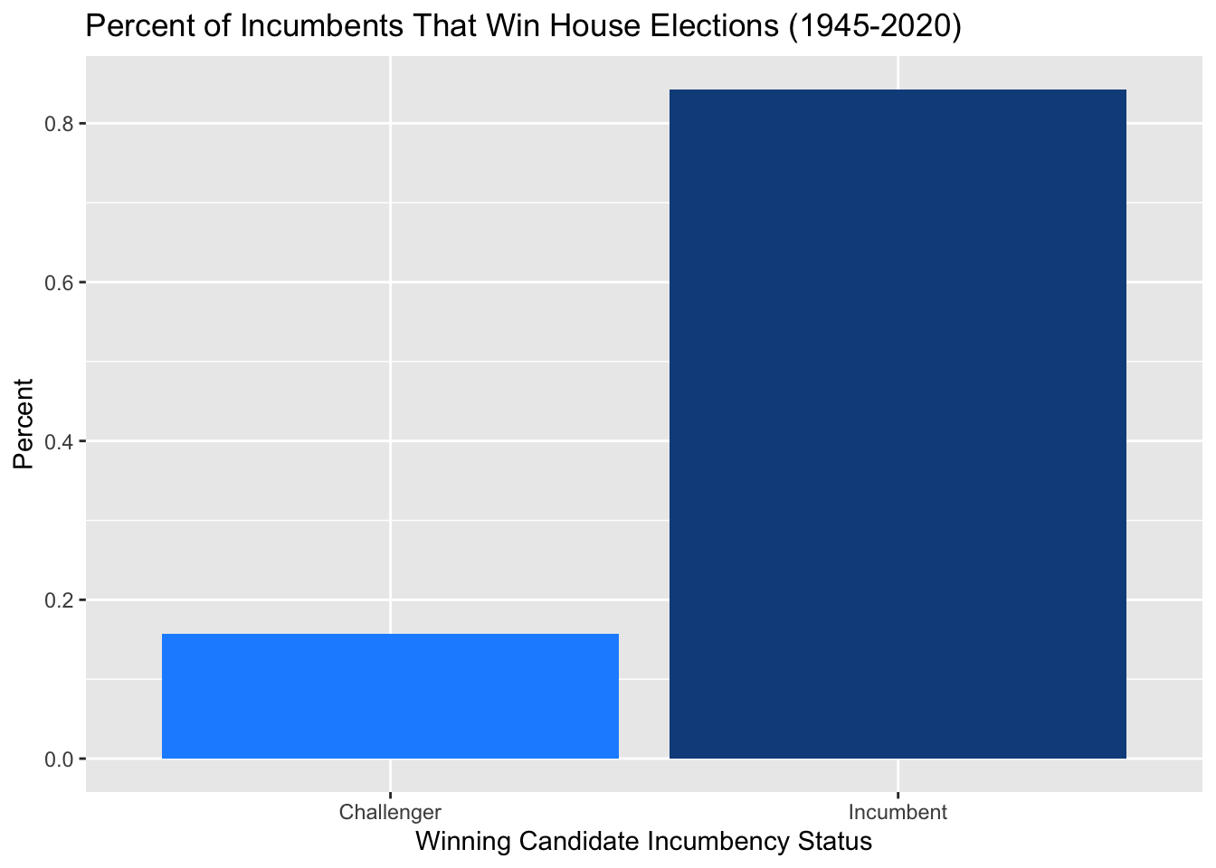
While this data is important at the district level, we learned about other incumbency phenomena that take place at a national level, such as the house flipping at midterm elections and the President’s party losing seats. Despite this incumbency data surely boasting high predictive power at the district-level, it does not provide much to us on a national-level. In a similar vein, however, rather than looking at the House majority incumbent from the year before, we can use the previous election’s vote share and seat share to predict that of the following election. I created lagged variables for both of these variables and will incorporate them into my final model, along with the President’s party variable that I previously mentioned.
The final variable I will be using in my model is an indicator variable for if the election takes place in a midterm year or not. From our discussions and readings, we know that different types of voters come out for midterm elections than presidential elections. We also learned in class that many Americans do not even know who their representative is. Those who vote in a midterm year are likely more involved politically and stay up-to-date with the news. I also will be interacting this term with the president’s party variable with the thought that it could account for some of the seat flipping that we historically see. Since 1955, every house flip has been the result of a midterm election (Reuters). This interaction term can account for the additional incumbent losses that occur during midterms but not during election years.
Throughout our time this semester, we have also worked with multiple other district-level variables that I will not be including in my model. We learned about advertising and the amount parties spend on advertising. In Gerber et al. 2011 the authors found that “televised ads have strong but short-lived effects on voting preferences”. With this in mind, along with in-class discussions about advertising data being unreliable and sometimes unavailable, I decided to forego using it in my model. Other district-level variables such as the cost of voting, ground campaigning efforts, and voter turnout I will not be adjusting to incorporate into my national model.
Formulas
Given all the data we have considered using this semester, and after many rounds of trial and error, I have created two final models. Below are the model equations and their corresponding regression tables using the national data that we are working with.
Midterm Models
After looking at both of those models that use data across all elections from 1960-2020, I wanted to see how these models would change if I limited the data to only midterm election years. As previously discussed, there is a different voting body in midterm elections versus presidential elections. In limiting the years I model on, I am hoping to improve their predictive power.
I removed the midterm indicator variable since the filter takes care of that, and also removed unemployment rate due to it causing a significant decrease in the adjusted r-squared. This left me with just the generic ballot support for democrats, the president’s party, and the previous democratic vote/seat share as independent variables. I ran this model on both vote share and seat share, and below are the results of this inquiry.
| Dependent variable: | |||
| D_majorvote_pct | |||
| (1) | (2) | (3) | |
| Generic Ballot Support - D | 0.671*** | 0.568*** | 0.515*** |
| (0.152) | (0.122) | (0.130) | |
| President Party - R | 3.290*** | 4.165*** | |
| (1.058) | (1.310) | ||
| Lag House Dem VS | 0.268 | ||
| (0.241) | |||
| Constant | 19.272** | 22.578*** | 10.626 |
| (7.461) | (5.876) | (12.225) | |
| Observations | 15 | 15 | 15 |
| R2 | 0.600 | 0.779 | 0.801 |
| Adjusted R2 | 0.569 | 0.742 | 0.747 |
| Residual Std. Error | 2.540 (df = 13) | 1.967 (df = 12) | 1.948 (df = 11) |
| F Statistic | 19.513*** (df = 1; 13) | 21.100*** (df = 2; 12) | 14.755*** (df = 3; 11) |
| Note: | p<0.1; p<0.05; p<0.01 | ||
| Dependent variable: | |||
| DemSeatShare | |||
| (1) | (2) | (3) | |
| Generic Ballot Support - D | 1.309*** | 1.206*** | 0.923*** |
| (0.287) | (0.290) | (0.224) | |
| President Party - R | 3.266 | 6.320*** | |
| (2.511) | (2.010) | ||
| Lag House Dem Seat Share | 0.493*** | ||
| (0.142) | |||
| Constant | -9.051 | -5.769 | -20.835* |
| (14.076) | (13.947) | (10.938) | |
| Observations | 15 | 15 | 15 |
| R2 | 0.616 | 0.663 | 0.840 |
| Adjusted R2 | 0.586 | 0.607 | 0.796 |
| Residual Std. Error | 4.792 (df = 13) | 4.669 (df = 12) | 3.364 (df = 11) |
| F Statistic | 20.851*** (df = 1; 13) | 11.826*** (df = 2; 12) | 19.236*** (df = 3; 11) |
| Note: | p<0.1; p<0.05; p<0.01 | ||
Both of these models have higher R-squared and adjusted R-squared values than their all-elections counterpart, with the vote share model boasting a 0.801 r-squared, and the seat share model having a 0.840.
The lag of Democratic house vote share in the vote share model is insignificant, but improves the R-squared and adjusted r-squared so I kept it in - as well as for consistency.
2022 Predictions
Using generic ballot data from FiveThirtyEight, Biden approval ratings from Gallup, and the 2022 Q3 unemployment rate from the BLS, I have predictions for each of the four models, including their 95% confidence interval, as noted by “lwr” and “upr”:
Democratic Vote Share using all years
##        fit      lwr     upr
## 1 50.20221 47.86202 52.5424
Democratic Seat Share using all years
##        fit     lwr      upr
## 1 50.50952 45.7082 55.31085
Democratic Vote Share using midterm years
##        fit      lwr      upr
## 1 47.85624 45.81439 49.89809
Democratic Seat Share using midterm years
##        fit      lwr      upr
## 1 46.38345 42.94734 49.81955
The predictions for the first two models that used data across all years are slightly higher than I would expect, specifically for the seat share. The seat share here is predicted to be split just about 50/50, which most experts do not believe will be the case this year. The models using data only from midterm elections, however, seem like they will more accurately predict this years election, at least in terms of being closer to what the experts are saying.
The two midterm-only models also have confidence intervals that do not cross 50%, meaning that they are 95% confident that the Democrats will not have more than 50% of the two-party vote share nor the seat share, meaning Republicans will win the house.
The model of Democratic Seat Share using midterm years predicts that Democrats will win 202 seats in the House, thus losing their majority, compared to the 219 that are predicted in the model that goes across all years.
In-Sample Testing
To validate this model, I conducted in-sample testing, predicting the vote and seat shares for each year within the model. I took these predictions and plotted them against the actual vote and seat shares in those years, producing the following graphs. The R-squared value of each model is also reflected on the plot. An R-squared of 1 would mean the model perfectly predicts the outcome.
In each graph I also added the 2022 predictions from the regression models. While the second model had the highest R-squared in its in-sample validation, based on what we know about the expert forecasts for this year’s election it seems a bit too high of a prediction. This prediction of a 50.50952 seat share for democrats is equivalent to 220 seats for Democrats. The fourth model had the lowest R-squared for its validation, but it had the highest R-squared out of all four regressions.
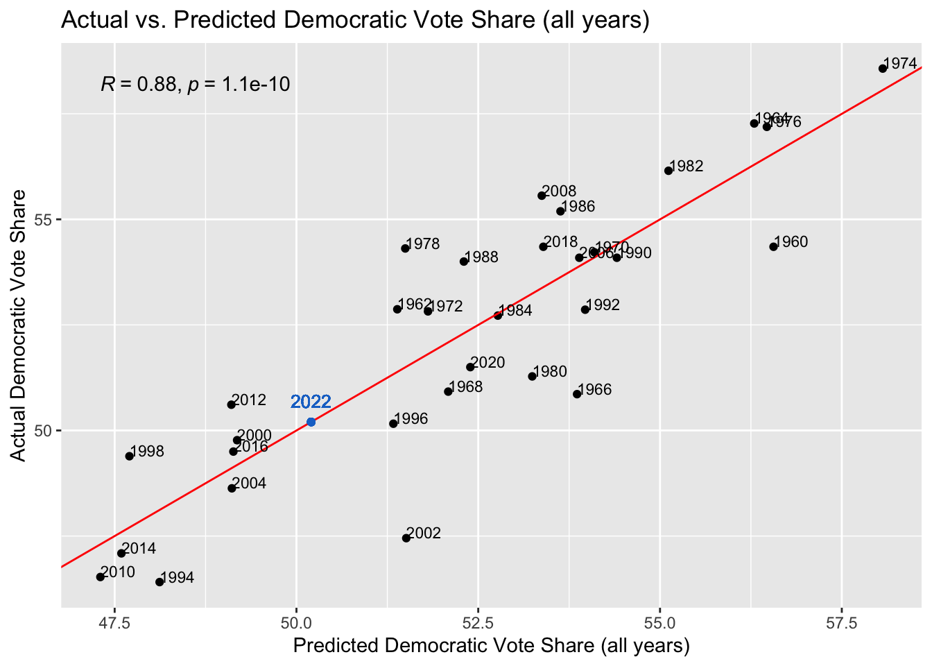
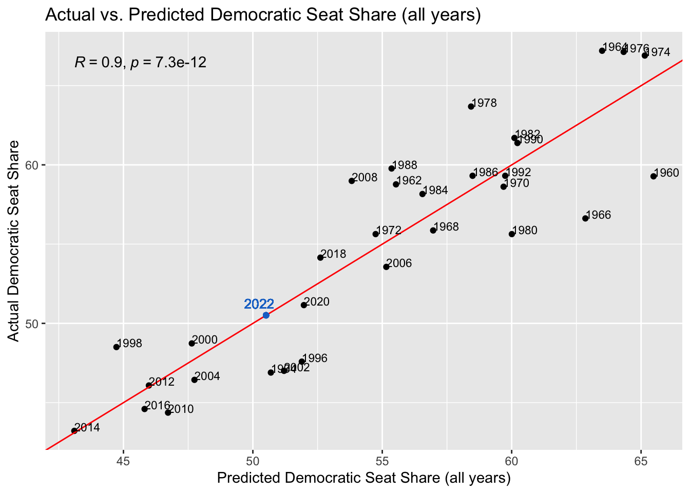
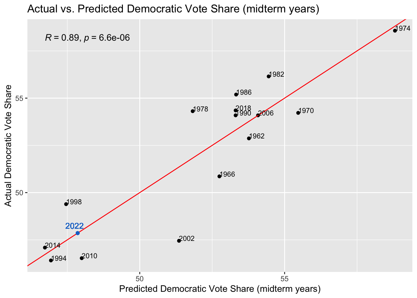
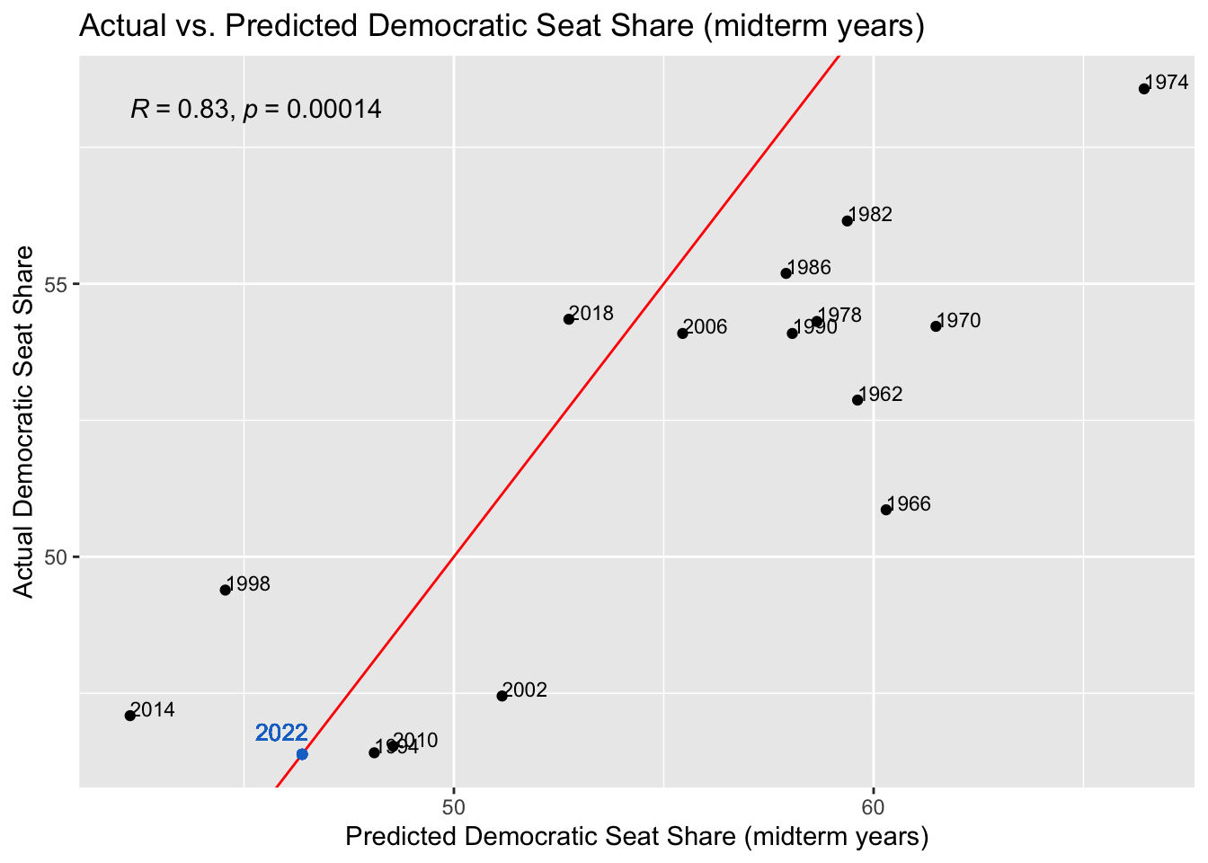
Looking at these plots, they all have fairly high R-squareds, which instills confidence into our predictions. Surprisingly, the seat share across all years has the highest R-squared of 0.9, when its prediciton of the democrats winning 220 seats seemed very off. Both vote share models have similar accuracy, with the midterm years one having an R-squared of 0.88 and the all years one having an R-squared of 0.89. The midterm years seat share model has the lowest accuracy, with an R-squared of 0.83, which is still high, but relative to the others, low.
Conclusion
The chart below shows my results from the seat share models and compares it to the current house make-up.
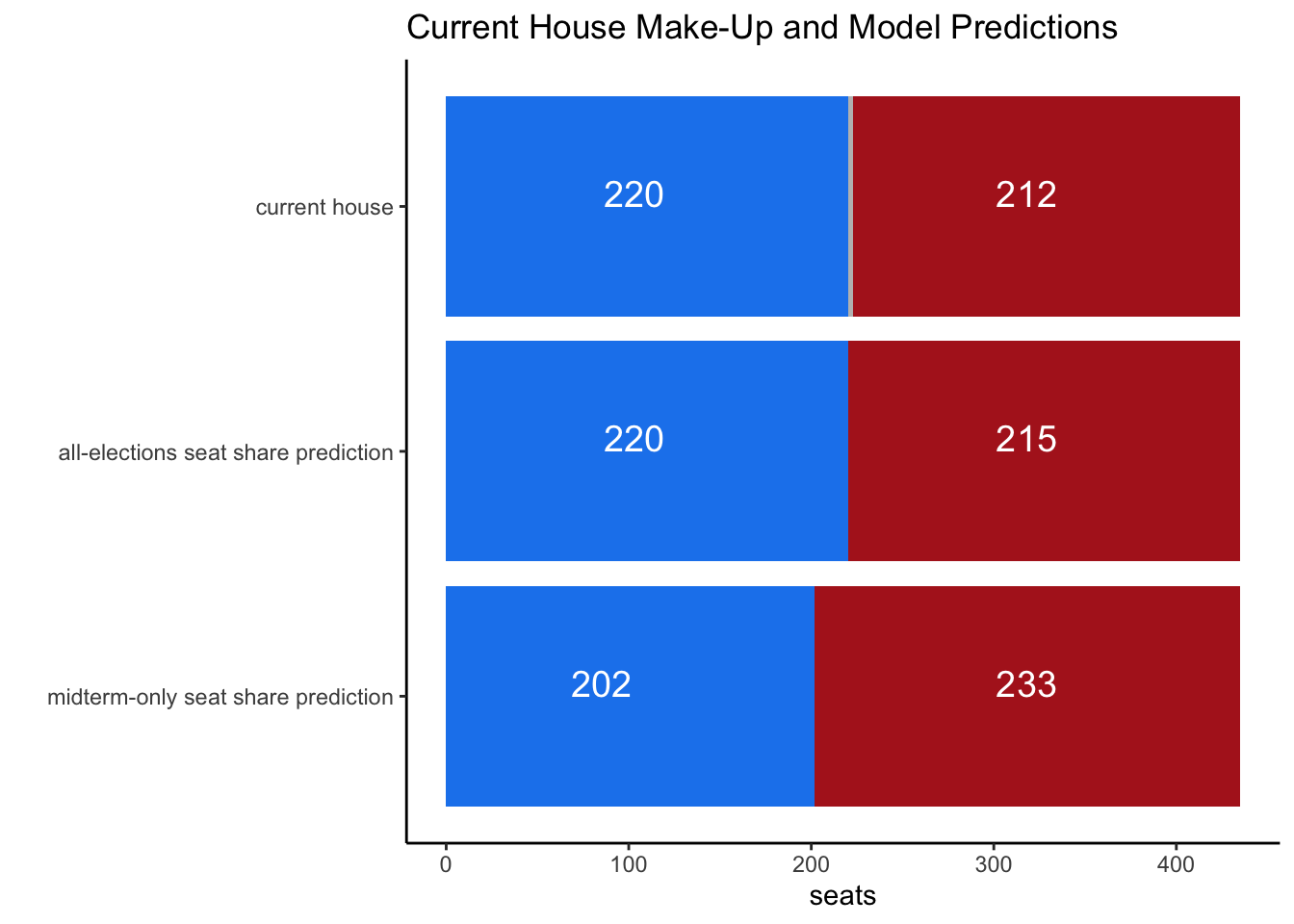
In conclusion, these models seem to suggest a close race. The models that use data across all elections predict a near equal 50/50 split in both vote share and seat share, while the midterm-only models slightly favor Republicans and predict them winning the house with 202 seats.
Throughout this class we have learned all sorts of modelling techniques and taken close looks at various independent variables to include. While it is impossible to know what will certainly happen on election day and predict exactly how everyone will vote, these forecasting methods will hopefully get us close. I look forward to reflecting on these models and methods after seeing how they performed.