on
Post-Election Reflection
This blog is part of a series related to Gov 1347: Election Analytics, a course at Harvard University taught by Professor Ryan D. Enos.
On Tuesday, November 8th, eligible Americans voted in the midterm elections for candidates who will make up the 118th Congress. As of today – November 21st, 2022 – the votes are still being counted leaving the final makeup of the Congress still up in the air, but the power of the House and Senate already decided. The Democrats have control of the Senate, whether it be a 50/50 split with Democratic Vice President Kamala Harris casting the decisive vote, or a 51/49 split with Democrats in control is up to the run-off election that will take place in December in Georgia. The House is in Republican control, but the predicted “red wave” that was expected in this year’s election never reached fruition. Prior to the election, we had created forecasting models in an attempt to determine who would win the House of Representatives, at the district-level, national-level, or both. In this post I will reflect on the predictions made, my model’s performance, and comment on the election overall.
Using the knowledge I gained this semester about election forecasting, I created multiple models to predict the outcome of the 2022 House of Representatives election. I looked at both seat share and vote share, and created two models for each: one using data across all election years, and one using the data for only midterm years. We had the opportunity to work with both national-level and seat-level data, but all of my final models used the data at the national-level for reasons I outlined in my Final Prediction Blog.
As a refresher, here are the predictions from my four models and the actual results of the election as of November 21st, 2022:
Model 1: Democratic Vote Share using all years \(\hat{Dem Vote Share}\) = 50.20% , 95% CI (47.86, 52.54) y = 47.59%
Model 2: Democratic Seat Share using all years \(\hat{Dem Seat Share}\) = 50.51% , 95% CI (45.71, 55.31) y = 49.30%
Model 3: Democratic Vote Share using midterm years \(\hat{Dem Vote Share}\) = 47.86% , 95% CI (45.81, 49.90) y = 47.59%
Model 4: Democratic Seat Share using midterm years \(\hat{Dem Seat Share}\) = 46.38% , 95% CI (42.95, 49.82) y = 49.30%
To start assessing the post-election accuracy of these models and reflect on their prediction capabilities, I have created four graphs below with the actual versus predicted results each year. In my Final Prediction Blog, these graphs had the 2022 predictions as a point along the regression line of the model with both the x and y value equaling the model’s prediction for the 2022 election. If its prediction had been completely accurate, this point would have stayed along the regression line. In the plots below, I have added a blue point that represents the actual election results as of November 21st, 2022, when 430 of the House seats have been decided. According to the Cook Political Report, Democrats have won 212 seats at this point, and Republicans have won 218 - a democratic seat share of 49.30%. The Cook Political Report also has counted a total of 50,464,746 votes for Democrats versus 53,948,354 for Republicans - giving a democratic vote share of 47.59%. In the graphs below, our predicted values have not changed since the models have not been adjusted at all from the final prediction, however the new y-value of the point shows the actual outcome. The distance between this point and the regression line shows the accuracy of our prediction, with a point closer to the line representing results that came very close to our prediction, and points further from the line representing a less-accurate prediction.
Model 1
\[ Democratic Vote Share = \beta_0 + Generic Ballot Democrat\beta_1 + Lag House Dem Vote Share\beta_2 + President Party R\beta_3 + President Approval\beta_4 + Midterm\beta_5 + Unemployment Rate\beta_6 + President Party R * Midterm\beta_7 + President Party R * Unemployment\beta_8 \]
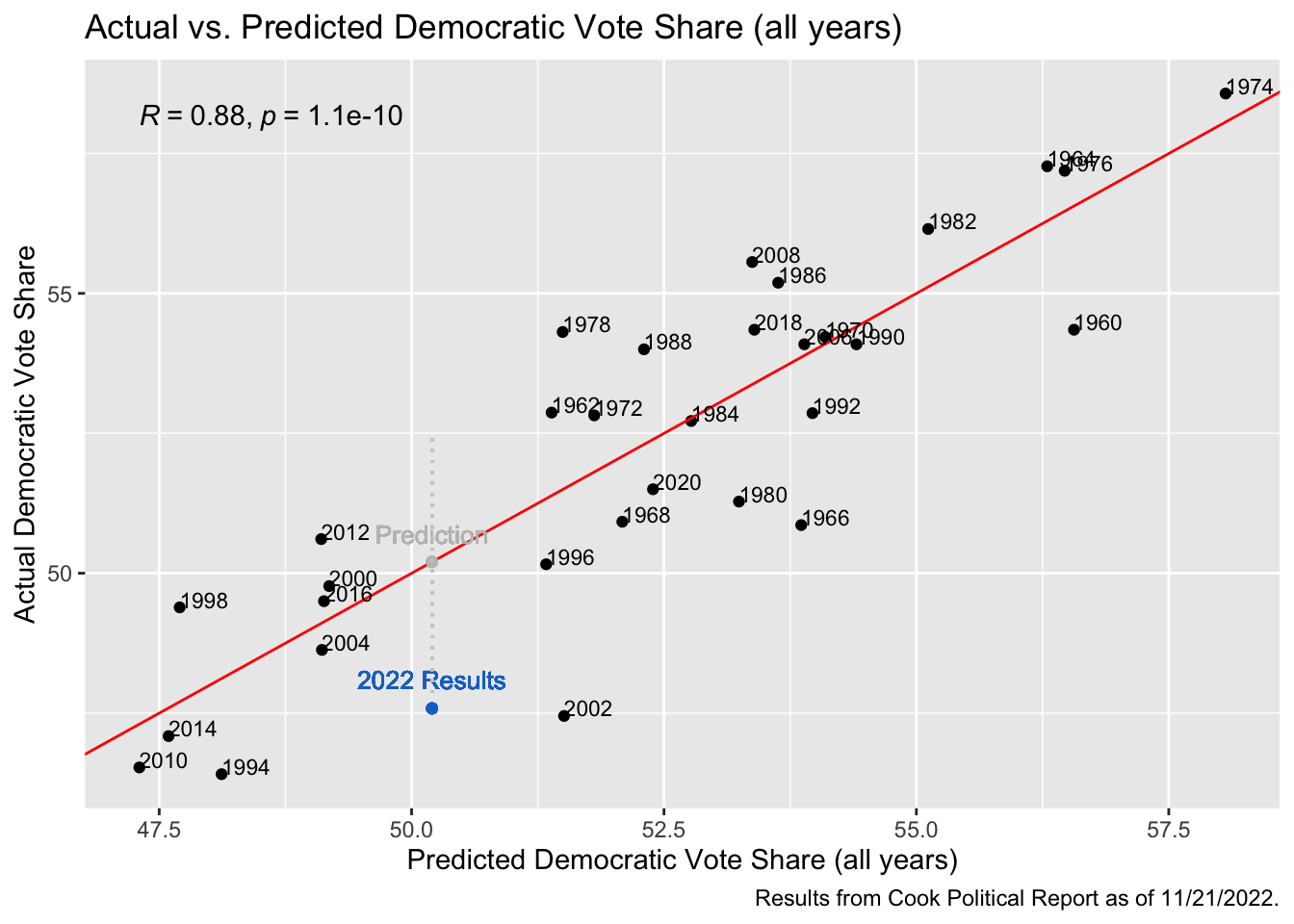
The graph above shows the model for vote share across all election years, both midterm and presidential. As we can see, the predicted vote share for the 2022 House was 50.2022%, or practically a tie between the Democrats and Republicans. We know that in recent history it is not uncommon for the vote share to be relatively close, even if one party comes away winning the majority of the seats – or in the case of a presidential election, the electoral votes – so this prediction seemed reasonable prior to the election. The actual democratic vote share was around 47.6%, which fell just outside of my prediction’s 95% Confidence Interval of (47.8, 52.54) that is represented by the grey dotted line on the plot. The fact that the actual vote share was not in the 95% confidence interval puzzles me a bit, as it makes me question whether this election fell to an extreme, or if this model was not the best predictor of the election since we would have hoped the error margins would be wide enough to capture this result. Despite these questions and falling outside of the confidence interval, my prediction is actually not that far off from the actual results, overestimating the vote share by 2.6122 percentage points.
Model 2
\[ Democratic Seat Share = \beta_0 + Generic Ballot Democrat\beta_1 + Lag House Dem Seat Share\beta_2 + President Party R\beta_3 + President Approval\beta_4 + Midterm\beta_5 + Unemployment Rate\beta_6 + President Party R * Midterm\beta_7 + President Party R * Unemployment\beta_8 \]
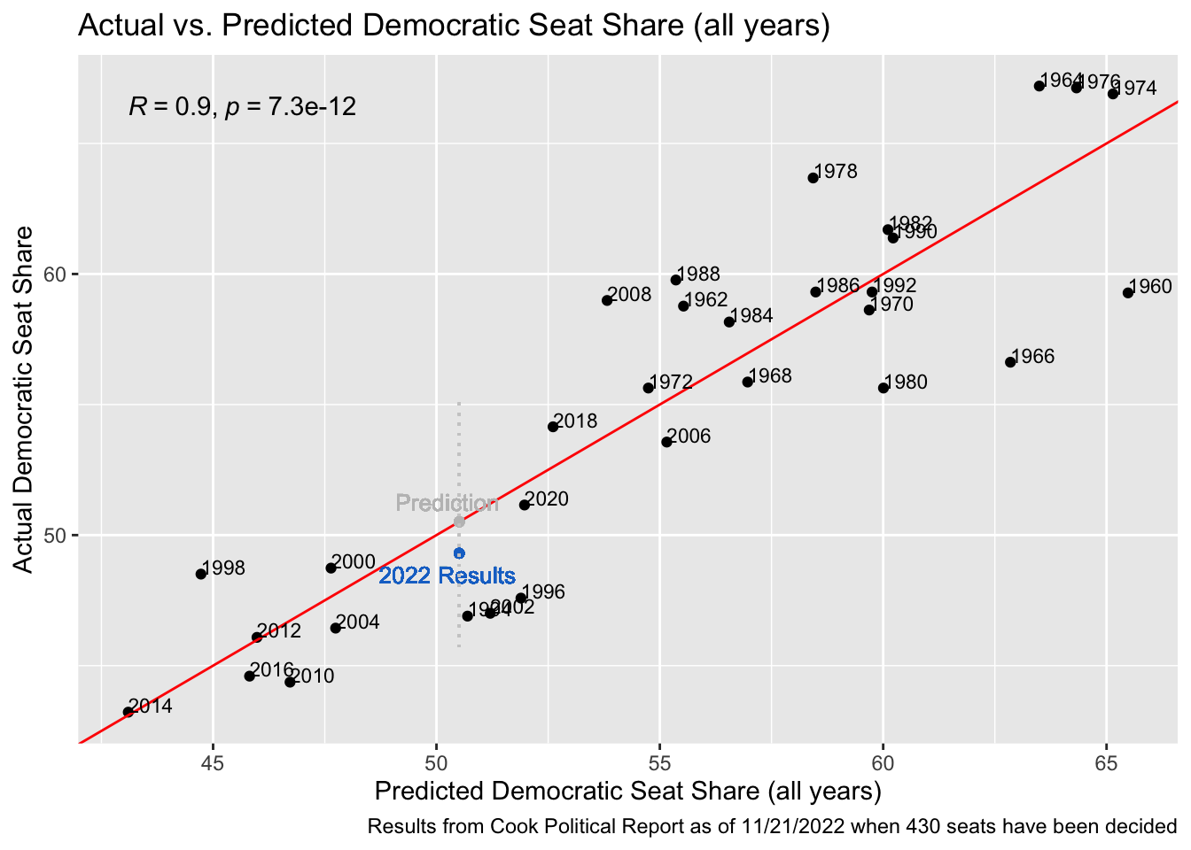 This model of seat share using data across all the election years fared much better than the one above, and produced a prediction that was very close to the results we actually saw, with the model overestimating the seat share by just 1.21 percentage points. In this model, the results also fell within the 95% confidence interval, unlike above. In my final election prediction blog, I noted that this model had the highest R-squared value, and these results resemble that accuracy.
Model 3
\[ Democratic Vote Share = \beta_0 + Generic Ballot Democrat\beta_1 + Lag House Dem Vote Share\beta_2 + President Party R\beta_3 \]
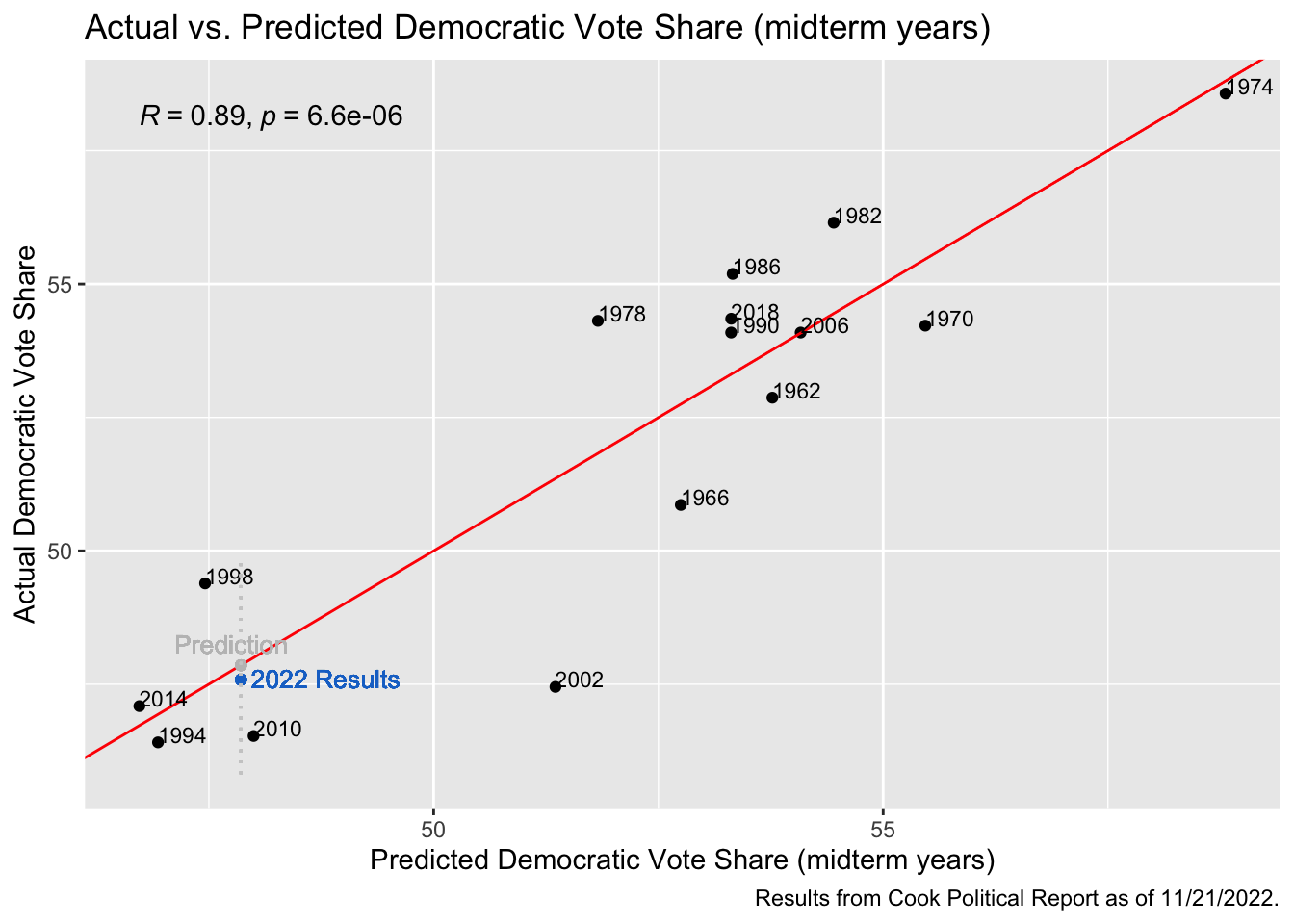
In the graph above, this model used only the midterm election years to regress on Democratic vote share and the results were extremely accurate. This model also had a high R-squared of 0.89, and it only overestimated the results by 0.27 percentage points. This was the most accurate prediction out of all four models, which surprised me a bit. In my initial predictions, I thought that these midterm year models would be less predictive, as they have fewer data points to work off of, and included fewer independent variables. While this midterm model was an accurate predictor, the other midterm model did not perform as well.
Model 4
\[ Democratic Seat Share = \beta_0 + Generic Ballot Democrat\beta_1 + Lag House Dem Seat Share\beta_2 + President Party R\beta_3 \]
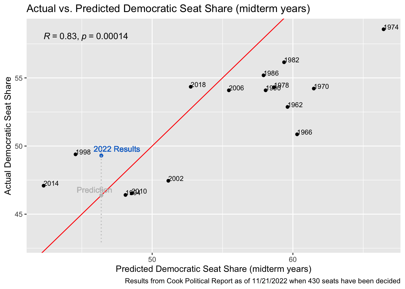
This midterm model underestimated the actual democratic seat share of the election by 2.92 percentage points. This was the only model that underestimated the dependent variable, however the prediction did still fall within the 95% confidence interval. This was the largest percentage-point difference between the prediction and the result across all four of the models, but I did expect this as the R-squared value is also the lowest of the four.
There are a few different reasons as to why my models may have been off, although it is hard to tell what may have caused any errors for certain. Incumbency variables did not favor democrats, and we can see the coefficients on President’s Party are relatively large and negative. Since this year the elections did not experience a “red wave” as was predicted, these incumbency variables may have taken away from the Democratic vote share more than they should have. I also believe my models could have been negatively affected by the inclusion of the President’s approval rating. This variable was not significant in the seat share model (Model 2), and only significant at the 0.1 level in the vote share model (Model 1). Similar to the coefficients with the president’s party, these coefficients were also negative and fairly high, taking away from Democratic votes and seats more than I probably should have allowed it to.
Looking at the results across all four models, it seems that using only the midterm years’ model for democratic vote share is more predictive than if we had used the model that spans all elections, while we see the opposite for democratic seat share - with the more predictive model being the one that uses all the elections. One reason I speculate this may be is because there is a different voter population during midterm years than election years, which has a strong affect on the vote share while the seats are more representative of the areas demographics. The number of voters in midterm years differs dramatically from the number that vote in election years - with presidential election years generating turnouts of around 50-60% and midterm elections only generating about 40% turnout. Since the number of voters participating differs between the two, it may be harder for the models that use all the years’ data to accurately predict the vote share down to a hundredth of a percentage point, as we are looking at here. If this speculation is somewhat correct, this would mean that incorporating voter turnout in to the model may have improved the accuracy. I will check this below by running the vote share model across all years and adding turnout as an independent variable to see if this improves the accuracy of the model.
| Dependent variable: | ||
| D_majorvote_pct | ||
| (1) | (2) | |
| Generic Ballot Support - D | 0.229** | 0.246** |
| (0.082) | (0.088) | |
| Lag House Dem VS | 0.426*** | 0.427*** |
| (0.119) | (0.120) | |
| President Party - R | -6.339** | -6.054* |
| (2.879) | (2.961) | |
| President Approval Rating | -5.435* | -5.485 |
| (3.155) | (3.203) | |
| Midterm Year | -4.644*** | -5.561*** |
| (1.053) | (1.866) | |
| Unemployment Rate | -0.690** | -0.678** |
| (0.307) | (0.312) | |
| President Party - R * Midterm Year | -0.054 | |
| (0.090) | ||
| President Party - R * Unemployment | 6.793*** | 6.839*** |
| (1.565) | (1.590) | |
| Constant | 0.793* | 0.731 |
| (0.424) | (0.443) | |
| Constant | 27.238*** | 29.460*** |
| (7.042) | (8.049) | |
| Observations | 31 | 31 |
| R2 | 0.767 | 0.771 |
| Adjusted R2 | 0.682 | 0.673 |
| Residual Std. Error | 1.830 (df = 22) | 1.857 (df = 21) |
| F Statistic | 9.051*** (df = 8; 22) | 7.852*** (df = 9; 21) |
| Note: | p<0.1; p<0.05; p<0.01 | |
Adding turnout to the model decreases the adjusted R-squared and it is an insignificant variable, however I will estimate a prediction using this model anyways to see how it performs. In order to make a prediction using the turnout model, I have estimated turnout for 2022 using the estimated 2021 citizen age voting population (CVAP) and the number of counted votes for 2022 as reported by the Cook Political Report on November 21st, 2022. This estimates the turnout to be around 41%, which falls in line with our typical midterm election turnout numbers, and we will proceed with using it despite some shortfalls that may result from this loose estimate.
##        fit      lwr      upr
## 1 52.36448 44.50132 60.22765
Looking at the prediction using this model, we see that the point estimate comes up with a democratic vote share of 52.36%, compared to the 50.20% we predicted in the model without turnout. This is even farther away from the actual results of the 2022 election, and therefore discredits my hypothesis that turnout could account for the difference in the vote share across all years model versus the model that only looks at midterm years.
Another hypothesis that I have as to how these models could be improved upon is that I did not account for any shocks, which may have made a bigger difference this year than in previous history. In class, we looked at shocks such as Dobbs v. Jackson on the generic ballot, as well as discussing other shocks such as the Clinton emails, and inflation. In that week’s investigation, we found that shocks did not have lasting effects on voter behavior, and often were not big enough issues to sway a significant amount of voters one way or another. This year may have been different. The Dobbs v. Jackson decision is a landmark in taking away women’s rights to health care, and this is something that is not forgotten easily. While other shocks may not have had lasting effects – and we even saw the Dobbs decision’s effect on the generic ballot dwindle over time – I think this may have been a stronger factor in voter’s decisions than I would have thought. This may have brought new voters to the polls, brought a different demographic of voters to the polls, or swayed voters more liberal, thus increasing the share of President’s party votes in this midterm year. If I possessed the data to do so, I would try to quantify this shock and measure its effect on the various models. I would do this by possibly polling voter’s stance on the issue, or asking voters for a key issue that led them to go to the polls on election day. This could possibly give us a measure of the importance of the issue to a sample of voters and we could add this to the model. Additionally, in relation to both the Dobbs decision and other trends, I would hypothetically like to incorporate demographic data on voter turnout to analyze the population that did vote. I think data such as youth turnout would be especially predictive this year, as we know younger generations of voters tend to be more left-leaning.
While we cannot access this demographic turnout data at this point in the election, we can try to analyze this election more like a presidential election year than a midterm one. We learned that in most midterm years, the President’s party will lose a lot of seats in the House of Representatives, and receive less vote share, and this was expected to happen again this year. However, as mentioned, this trend did not persist this year. While the limitations and difficulties with trying to measure the effect of a shock on an election remain, I will try to test the more general hypothesis that this year behaved less like a midterm year by removing the midterm year indicator variable and its interaction with the President’s party variable. I will repeat the steps from above and re-evaluate the performance of the model.
| Dependent variable: | ||
| D_majorvote_pct | ||
| (1) | (2) | |
| Generic Ballot Support - D | 0.229** | 0.246** |
| (0.082) | (0.088) | |
| Lag House Dem VS | 0.426*** | 0.427*** |
| (0.119) | (0.120) | |
| President Party - R | -6.339** | -6.054* |
| (2.879) | (2.961) | |
| President Approval Rating | -5.435* | -5.485 |
| (3.155) | (3.203) | |
| Midterm Year | -4.644*** | -5.561*** |
| (1.053) | (1.866) | |
| Unemployment Rate | -0.690** | -0.678** |
| (0.307) | (0.312) | |
| President Party - R * Midterm Year | -0.054 | |
| (0.090) | ||
| President Party - R * Unemployment | 6.793*** | 6.839*** |
| (1.565) | (1.590) | |
| Constant | 0.793* | 0.731 |
| (0.424) | (0.443) | |
| Constant | 27.238*** | 29.460*** |
| (7.042) | (8.049) | |
| Observations | 31 | 31 |
| R2 | 0.767 | 0.771 |
| Adjusted R2 | 0.682 | 0.673 |
| Residual Std. Error | 1.830 (df = 22) | 1.857 (df = 21) |
| F Statistic | 9.051*** (df = 8; 22) | 7.852*** (df = 9; 21) |
| Note: | p<0.1; p<0.05; p<0.01 | |
fit lwr upr1 48.81535 43.23659 54.39412
In removing these two variables, the adjusted R-squared decreases by 0.26, which is a fairly significant amount. In addition, most of the variables also lose their significance after removal. However, the point prediction using this model is 48.82% of the democratic vote share, compared to the 50.20% in our original model. This is much closer to the actual democratic vote share of 47.6%, but the 95% confidence interval also gets wider when adjusting the model in this way. While I cannot say for sure that this election acted differently than other midterm elections because of the shock of Dobbs v. Jackson, the inclusion of the midterm variable does seem to shift the data more positively towards Democrats, surpassing the vote share we actually see.
My midterm vote share model (Model 3) surprised me a bit with its accuracy, as it only used 3 independent variables: generic ballot, president’s party, and a lag of the vote share from the previous election. What made it even more surprising was the fact that only generic ballot and president’s party were significant, yet the model still produced an extremely accurate result. This may have been more due to luck that the actual capability of the model.
Looking back at all of my models, there are a few areas that I would have liked to improve them. For starters, I used only unemployment rate as an economic variable for the first two models. In creating these models, I tried different variations of GDP, CPI, and RDI, but none of these variables ever had a positive impact on the models and usually reduced the adjusted R-squared value. I mostly was looking at these values in Quarter 3 (or Quarter 7 of the two year cycle) and there may be something wrong with this time frame that results in its lack of predictability. While I am not sure if there is a quick, streamlined process to test these economic variables against the vote share/seat share, I would like to regress each quarter’s average against the dependent variables, and possibly do other time periods as well, such as the month before an election or 6 months before. I would like to then take the time frame that is most predictive, as measured by an R-squared value, and try to incorporate that into the models. There was also discussion in our class about consumer sentiment as an economic indicator, and its predictive strength. This could be another economic variable worth looking into to improve the models.
Overall, my models performed okay but there is always room for improvement. I think some key issues that should be addressed with them would be the inclusion of incumbency variables, the lack of economic variables, and the addition of the Dobbs v. Jackson shock. I could also look at different modeling techniques other than linear regression, like a random forest or ensemble model. I also believe these models could have performed better if there had been a way to know that this year would behave more like a presidential year than a midterm year. Other than these considerations, I am happy with the performance of my models and would like to see how they work out in other modern elections.